
Introduction to TensorFlow Probability
Goal
In the previous articles, we discuss the concepts of Bayesian Neural Network (BNN) and the mathematical theories behind. For those who are new to BNN, make sure you have checked the links below.
Bayesian Neural Network explains the uncertainties from the model and provides the distributions over the weights and…towardsdatascience.com
The meaning of Prior, Posterior, Bayes’ Theorem, Negative Log-Likelihood, KL Divergence, Surrogate, Variational…towardsdatascience.com
Today, we will explore probabilistic programming using TensorFlow-Probability to implement the BNN model. From this article, you will learn how to use TensorFlow Probability to
- build different distributions and sample from them.
- use the bijective function to transform the data.
- combine the probabilistic layers with Keras to build the BNN model.
- inference and illustrate different types of uncertainties.
What is TensorFlow Probability?
TensorFlow Probability (TFP) is a library for probabilistic reasoning and statistical analysis in TensorFlow. It provides integration of probabilistic methods with deep networks, gradient-based inference using automatic differentiation, and scalability to large datasets and models with hardware acceleration (GPUs) and distributed computation. In fact, TFP is a comprehensive tool that consists of many modules including probabilistic layers, variational inference, MCMC, Nelder-Mead, BFGS and etc. But I am not going to drill down all of the modules and only some of them will be picked and demonstrated. If you would like to know more details, do check the tech doc below.
Distributions
As the probabilistic programming package, one of the key modules TFP supports would be different kinds of statistical distributions. To be honest, I have to say TFP has done a pretty good job and it covers quite a lot of distributions (including lots of them I have no ideas what they are haha). After the counting, I found there are 117 distributions provided as of Oct 2021. I am not going to list their names here. For more details, you can check their api docs here.
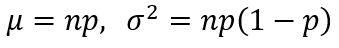
And today, I would like to share some of the functionalities that I think are useful and share with you guys. In the following, I will use Binomial as the illustration.
import tensorflow_probability as tfp
tfd = tfp.distributions
n = 10000
p = 0.3
binomial_dist = tfd.Binomial(total_count=n, probs=p)
1. Sample Data
Let say we would like to draw 5 samples from the binomial distribution we just created. You only need to use the method sample and specify the number of samples you would like to draw.
binomial_dist.sample(5)
<tf.Tensor: shape=(5,), dtype=float32, numpy=array(
[3026., 3032., 2975., 2864., 2993.], dtype=float32)>
2. Summary Statistics
Another cool feature is to obtain the summary statistics. For some simple distribution like Binomial, we can easily derive the statistics by
However, for some complicated distributions, it may not be an easy task to calculate the statistics. But now you can simply leverage the tools.
mu = binomial_dist.mean()
std = binomial_dist.stddev()
print('Mean:', mu.numpy(), ', Standard Deviation:', std.numpy())
Mean: 3000.0 , Standard Deviation: 45.825756
3. Probability Density Function (PDF)
To find the PDF for a given x, we can use the method prob.
x = 3050
pdf = binomial_dist.prob(x)
print('PDF:', pdf.numpy())
PDF: 0.004784924
import matplotlib.pyplot as plt
fig = plt.figure(figsize = (10, 6))
x_min = int(mu-3*std)
x_max = int(mu+3*std)
pdf_list = [binomial_dist.prob(x) for x in range(x_min, x_max)]
plt.plot(range(x_min, x_max), pdf_list)
plt.title('Probability Density Function')
plt.ylabel('$pdf$')
plt.xlabel('$x$')
plt.show()

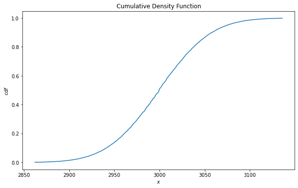
4. Cumulative Density Function (CDF)
To find the CDF for a given x, we can use the method cdf.
x = 3050
cdf = binomial_dist.cdf(x)
print('CDF:', cdf.numpy())
CDF: 0.865279
fig = plt.figure(figsize = (10, 6))
x_min = int(mu-3*std)
x_max = int(mu+3*std)
cdf_list = [binomial_dist.cdf(x) for x in range(x_min, x_max)]
plt.plot(range(x_min, x_max), cdf_list)
plt.title('Cumulative Density Function')
plt.ylabel('$cdf$')
plt.xlabel('$x$')
plt.show()
5. Log-Likelihood
The last method I would like to introduce would be log_prob. This is used to calculate the log-likelihood. From the previous two articles, I thought everyone would have a sense that how important this is since we would always use it as the loss function. So to find the log-likelihood, we simply call
x = 3050
l = binomial_dist.log_prob(x)
print('Log-likelihood:', l.numpy())
Log-likelihood: -5.342285
fig = plt.figure(figsize = (10, 6))
x_min = int(mu-3*std)
x_max = int(mu+3*std)
l_list = [binomial_dist.log_prob(x) for x in range(x_min, x_max)]
plt.plot([j for j in range(x_min, x_max)], l_list)
plt.title('Log-Likelihood')
plt.ylabel('$l$')
plt.xlabel('$x$')
plt.show()

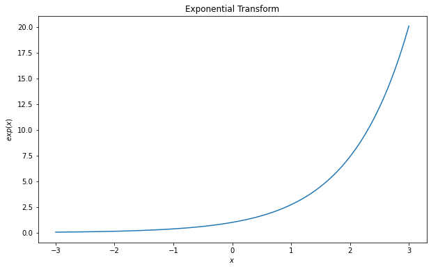
Bijectors
Bijector is the term named by TensorFlow and basically, it refers to the bijective transformations. By definition, bijective transformation is a function between the elements of two sets, where each element of one set is paired with exactly one element of the other set, and each element of the other set is paired with exactly one element of the first set.
To me, I will consider bijectors as the ready-to-use data transformation functions. You can find many common functions here such as Log, Exp, Sigmoid, Tanh, Softplus, Softsign and etc.
You can simply call the bijector with the following codes.
tfb = tfp.bijectors
exp = tfb.Exp()
To apply the transformation, you just have to pass the values to the object.
import numpy as np
x = np.linspace(-3, 3, 100)
y = exp(x)
fig = plt.figure(figsize = (10, 6))
plt.plot(x, y)
plt.title('Exponential Transform')
plt.ylabel('$exp(x)$')
plt.xlabel('$x$')
plt.show()
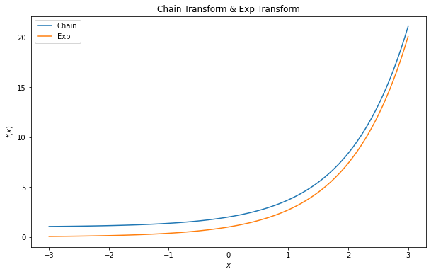
Just one tip I would like to share, there is a bijector named Chain, which is used to apply a sequence of bijectors. For example, if we would like to pass x to the softplus function and follow by the exp function. We can write like
exp = tfb.Exp()
softplus = tfb.Softplus()
chain = tfb.Chain([exp, softplus])
By doing so, it is equivalent to

x = np.linspace(-3, 3, 100)
y_chain = chain(x)
y_exp = exp(x)
fig = plt.figure(figsize = (10, 6))
plt.plot(x, y_chain, label = 'Chain')
plt.plot(x, y_exp, label = 'Exp')
plt.title('Exponential Transform')
plt.ylabel('$exp(x)$')
plt.xlabel('$x$')
plt.legend()
plt.show()
Layers
tfp.layers module sets up a user-friendly interface for developers to easily switch their models from Standard Neural Network into Bayesian Neural Network by replacing the original layers into probabilistic layers. In the following, I will list out some of the layers I often use for reference.
- DenseVariational: epistemic uncertainty
- IndependentNormal: aleatory uncertainty
- DistributionLambda: aleatory uncertainty
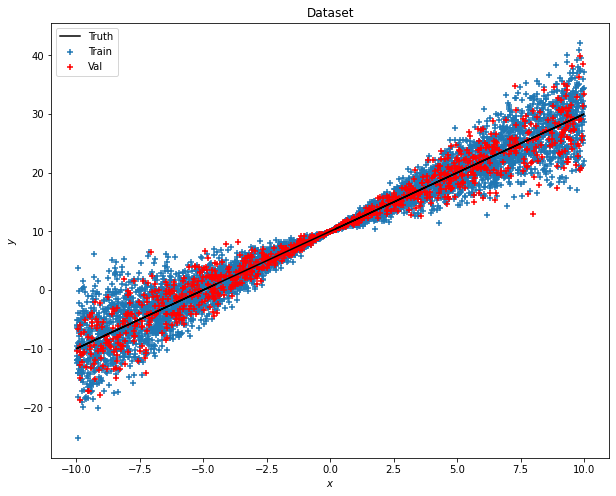
1. Create Dataset
So to train the BNN model, first things first, we have to create the dataset.
def create_dataset(n, x_range, slope=2, intercept=10, noise=0.5):
    x_uniform_dist = tfd.Uniform(low=x_range[0], high=x_range[1])
    x = x_uniform_dist.sample(n).numpy().reshape(-1, 1)
    y_true = slope*x+intercept
    eps_uniform_dist = tfd.Normal(loc=0, scale=1)
    eps = eps_uniform_dist.sample(n).numpy().reshape(-1, 1)*noise*x
    y = y_true + eps
    return x, y, y_true
n_train = 5000
n_val = 1000
n_test = 5000
x_range = [-10, 10]
x_train, y_train, y_true = create_dataset(n_train, x_range)
x_val, y_val, _ = create_dataset(n_val, x_range)
x_test = np.linspace(x_range[0], x_range[1], n_test).reshape(-1, 1)
The sample data is actually a linear fit with a heterogeneous variance along with the value of x. To better visualize, you can plot with the following codes.
def plot_dataset(x_train, y_train, x_val, y_val, y_true, title):
    fig = plt.figure(figsize = (10, 8))
    plt.scatter(x_train, y_train, marker='+', label='Train')
    plt.scatter(x_val, y_val, marker='+', color='r', label='Val')
    plt.plot(x_train, y_true, color='k', label='Truth')
    plt.title(title)
    plt.xlabel('$x$')
    plt.ylabel('$y$')
    plt.legend()
    plt.show()
plot_dataset(x_train, y_train, x_val, y_val, y_true, 'Dataset')
2. Standard Neural Network
Before training the BNN, I would like to make a Standard Neural Network as the baseline for comparison purpose.
import tensorflow as tf
tfkl = tf.keras.layers
# Model Architecture
model = tf.keras.Sequential([
    tfkl.Dense(1, input_shape = (1,))
])
# Model Configuration
model.compile(optimizer=tf.optimizers.Adam(learning_rate=0.01), loss=tf.keras.losses.MeanSquaredError())
# Early Stopping Callback
callback = tf.keras.callbacks.EarlyStopping(monitor='val_loss', patience=30, min_delta=0, mode='auto', baseline=None, restore_best_weights=True)
# Model Fitting
history = model.fit(x_train, y_train, validation_data=(x_val, y_val), epochs=1000, verbose=False, shuffle=True, callbacks=[callback], batch_size = 100)
As you may observe, the simple model only sets one Dense hidden layer and to check how’s the model performs, we can use the predict method.
y_pred = model.predict(x_test)
fig = plt.figure(figsize = (10, 8))
plt.scatter(x_train, y_train, marker='+', label='Train')
plt.plot(x_train, y_true, color='k', label='Truth')
plt.plot(x_test, y_pred, color='r', label='Predict')
plt.legend()
plt.title('Standard Neural Network')
plt.show()
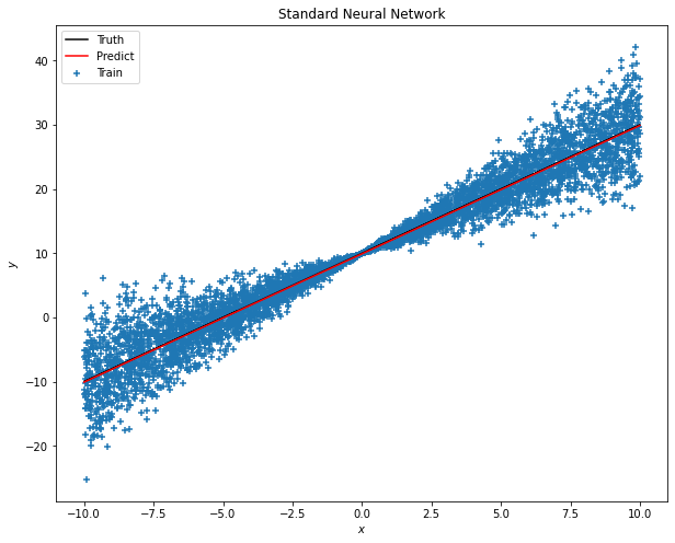
It seems that the prediction matches with the truth linear line as expected. However, using SNN cannot tell the uncertainty of the predictions.
3. Bayesian Neural Network
So it comes to the main dish. Let’s discuss the code step by step.
3.1 Model Architecture
tfpl = tfp.layers
model = tf.keras.Sequential([
    tfkl.Dense(2, input_shape = (1,)),
    tfpl.DistributionLambda(lambda t: tfd.Normal(loc=t[..., :1], scale=1e-3+tf.math.abs(t[...,1:])))
])
You may notice that we will have a Dense layer outputting two neurons. Can you guess what these two parameters are for? They are the mean and standard deviation that will be passed to the normal distribution we have specified in the DistributionLambda layer.
3.2 Model Configuration
negloglik = lambda y_true, y_pred: -y_pred.log_prob(y_true)
model.compile(optimizer=tf.optimizers.Adam(learning_rate=0.01), loss=negloglik)
As per our discussion in the previous articles, instead of the MSE, we will use negative log-likelihood for BNN. If you have no ideas what I am talking about, I highly recommend you go back to the previous two articles and get familiar with the concepts and theories first.
3.3 Train the Model
# Early Stopping Callback
callback = tf.keras.callbacks.EarlyStopping(monitor='val_loss', patience=300, min_delta=0, mode='auto', baseline=None, restore_best_weights=True)
# Model Fitting
history = model.fit(x_train, y_train, validation_data=(x_val, y_val), epochs=10000, verbose=False, shuffle=True, callbacks=[callback], batch_size = 100)
Nothing special here and basically everything is similar to the SNN setting so I will skip this part.
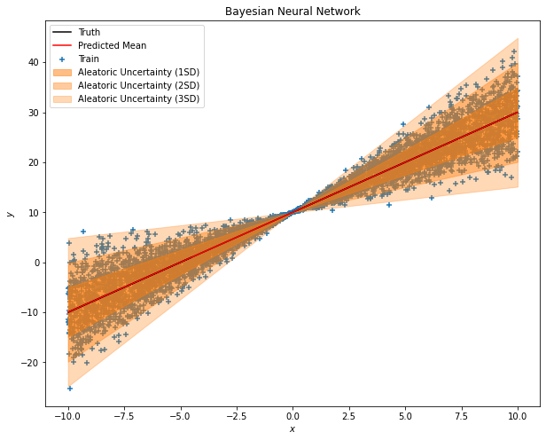
3.4 Prediction
The MOST VALUABLE code today is right here.
# Summary Statistics
y_pred_mean = model(x_test).mean()
y_pred_std = model(x_test).stddev()
By calling the mean and stddev function, you can now tell the uncertainty level of your prediction.
fig = plt.figure(figsize = (10, 8))
plt.scatter(x_train, y_train, marker='+', label='Train')
plt.plot(x_train, y_true, color='k', label='Truth')
plt.plot(x_test, y_pred_mean, color='r', label='Predicted Mean')
plt.fill_between(x_test.ravel(), np.array(y_pred_mean+1*y_pred_std).ravel(), np.array(y_pred_mean-1*y_pred_std).ravel(), color='C1', alpha=0.5, label='Aleatoric Uncertainty (1SD)')
plt.fill_between(x_test.ravel(), np.array(y_pred_mean+2*y_pred_std).ravel(), np.array(y_pred_mean-2*y_pred_std).ravel(), color='C1', alpha=0.4, label='Aleatoric Uncertainty (2SD)')
plt.fill_between(x_test.ravel(), np.array(y_pred_mean+3*y_pred_std).ravel(), np.array(y_pred_mean-3*y_pred_std).ravel(), color='C1', alpha=0.3, label='Aleatoric Uncertainty (3SD)')
plt.title('Bayesian Neural Network')
plt.xlabel('$x$')
plt.ylabel('$y$')
plt.legend()
plt.show()
Conclusion
See, you can now be able to distinguish the aleatoric uncertainty for the model outputs. Wait, then where is the epistemic uncertainty? I left this part for you guys to further explore. The tip is to replace the Dense layer with the DenseVariational layer. Go and try it out. =)
Comments
Post a Comment